Inspecting Parameters
Before running detection, it's useful to inspect the intermediate parameters (entropy, information content, and bin deviation) to understand what the algorithm sees. These are the building blocks of the detection rule.
The Three Parameters
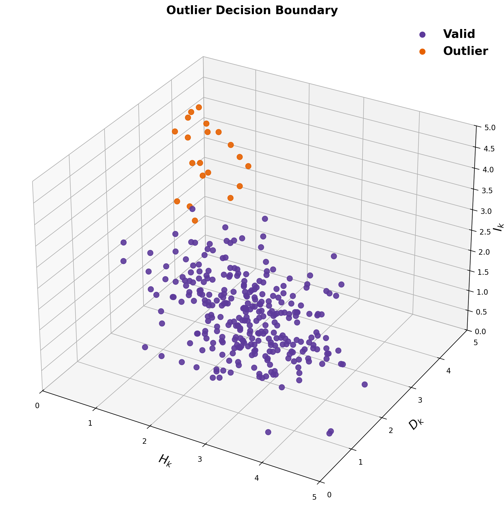
Valid readings (purple) cluster at high entropy, low deviation, low information. Outliers (orange) appear in the opposite corner.
1. Network Entropy
Shannon entropy measures how spread out the bin assignments are across the network. Low entropy means most sensors agree (readings cluster in one or two bins). High entropy means sensors disagree (readings spread across many bins).
import elwood_spatial as es

values = {"s1": 45, "s2": 48, "s3": 120, "s4": 42, "s5": 50}
bins = es.BinSpec.from_tuples([(0, 50), (51, 100), (101, 150), (151, 200)])

bin_indices = [bins.bin_index(v) for v in values.values()]
# => [0, 0, 2, 0, 0]

entropy = es.shannon_entropy(bin_indices)
print(f"Entropy: {entropy:.3f} bits")
# => Entropy: 0.722 bits  (low, most sensors agree on bin 0)

probs = es.bin_probabilities(bin_indices)
print(f"Probabilities: {probs}")
# => {0: 0.8, 2: 0.2}
During a smoke event, many sensors legitimately read high AQI, so entropy rises as readings spread across bins. The entropy ceiling S prevents false positives during these events: detection is suppressed when entropy is high.
2. Information Content
Information content Ik = −log2(pk) measures how "surprising" a sensor's bin is. A sensor in a bin that no other sensor occupies has maximum information. A sensor in the most common bin has low information.
# Which sensor is the most "surprising"?
for name, value in values.items():
    bi = bins.bin_index(value)
    ic = es.information_content(bi, bin_indices)
    print(f"{name}: value={value}, bin={bi}, information={ic:.3f} bits")

# s1: value=45,  bin=0, information=0.322 bits  (common bin)
# s2: value=48,  bin=0, information=0.322 bits
# s3: value=120, bin=2, information=2.322 bits  ← rare bin, high information
# s4: value=42,  bin=0, information=0.322 bits
# s5: value=50,  bin=0, information=0.322 bits
3. Bin Deviation
Bin deviation Dk = |Bk − mean(Bj)| measures how far a sensor's bin index is from the mean of its neighbors. A sensor reading "Hazardous" when all its neighbors read "Good" will have high bin deviation.
for name, value in values.items():
    bi = bins.bin_index(value)
    others = [bins.bin_index(v) for k, v in values.items() if k != name]
    bd = es.bin_deviation(bi, others)
    print(f"{name}: bin={bi}, bin_deviation={bd:.3f}")

# s1: bin=0, bin_deviation=0.500
# s3: bin=2, bin_deviation=2.000  ← far from neighbors' mean
4. All Parameters at Once
compute_network_metrics returns per-device entropy, information, and
bin deviation in a single call:
bin_indices_dict = {k: bins.bin_index(v) for k, v in values.items()}
metrics = es.compute_network_metrics(bin_indices_dict)

for device_id, m in metrics.items():
    print(f"{device_id}:  H={m['entropy']:.3f}  "
          f"I={m['information']:.3f}  "
          f"D={m['bin_deviation']:.3f}")
5. Understanding the Detection Rule
A sensor is flagged as an outlier only when all three conditions hold:
| Condition | What it means | Default |
|---|---|---|
| Ik ≥ θ | The sensor's reading is rare in the network | θ = 1.75 |
| H < S | The network overall shows agreement (not a widespread event) | S = 1.75 |
| Dk ≥ nbins / β | The sensor's bin is far from its neighbors' mean bin | β = 3.5 |
The conjunction of all three prevents false positives: high information alone isn't enough (maybe it's a real event), and low entropy alone isn't enough (maybe the sensor is just in an adjacent bin).
6. Theoretical Entropy Benchmarks
Use entropy_at_agreement to understand what entropy values to expect for
different levels of sensor agreement:
# What entropy to expect at different agreement levels?
for frac in [0.5, 0.75, 0.9, 1.0]:
    h = es.entropy_at_agreement(20, agreement_fraction=frac, n_bins=12)
    print(f"{frac:.0%} agreement among 20 sensors → H = {h:.3f} bits")

# 50% agreement → H = 3.170 bits  (high, lots of disagreement)
# 75% agreement → H = 1.963 bits  (moderate)
# 90% agreement → H = 1.028 bits  (low, strong consensus)
# 100% agreement → H = 0.000 bits (perfect agreement)
7. Coefficient of Variation as an Amendment
The information-theoretic detection rule operates on a single snapshot in time. In practice, it can be useful to amend the outlier list using the coefficient of variation (CV), a measure of how dynamic a sensor's readings have been over a recent time window (e.g. 24 hours).
CV is defined as the ratio of the standard deviation to the mean, expressed as a percentage:
from elwood_spatial.features import coefficient_of_variation

# CV = (std / mean) * 100
values = [150, 152, 148, 151, 149, 150, 150, 151]  # fairly stable
cv = coefficient_of_variation(values)
print(f"CV = {cv:.2f}%")
# => CV = 0.89%  (very low, sensor barely moving)

dynamic = [42, 85, 160, 120, 55, 200, 95, 70]  # actively changing
cv = coefficient_of_variation(dynamic)
print(f"CV = {cv:.2f}%")
# => CV = 53.6%  (high, sensor is responsive)
A sensor with low CV has reported nearly the same value for an extended period and may be stuck or flatlined. A sensor with high CV has been changing rapidly, which may indicate it is responding to a genuine environmental signal.
Adding outliers: identifying stuck sensors
If a sensor is reading a high value (e.g. AQI ≥ 200) but its CV over the past 24 hours is very low (e.g. ≤ 7.5%), this suggests it may be stuck at that value rather than responding to a real event. In this case, you might add the device to the outlier list even if the information-theoretic rule did not flag it, perhaps because the network around it is also disordered (high entropy), suppressing detection.
# After running detection, amend with CV to catch stuck sensors
import pandas as pd
from elwood_spatial.features import coefficient_of_variation

# Suppose these sensors were NOT flagged by the info-theoretic rule
# (perhaps network entropy was too high during the event)
# but they are reading very high AQI with suspiciously flat readings:

recent_readings = {
    "abc123": [310, 310, 310, 310, 310, 310, 310, 310],  # stuck at 310
    "def234": [295, 310, 280, 330, 305, 315, 290, 340],  # actively changing
}

cv_threshold = 7.5  # percent

for sensor_id, readings in recent_readings.items():
    cv = coefficient_of_variation(readings)
    if cv <= cv_threshold:
        print(f"{sensor_id}: CV={cv:.1f}% → stuck, adding to outlier list")
    else:
        print(f"{sensor_id}: CV={cv:.1f}% → dynamic, leaving alone")

# abc123: CV=0.0% → stuck, adding to outlier list
# def234: CV=6.8% → dynamic, leaving alone
Removing outliers: allowing dynamic sensors to resolve
Conversely, if a flagged sensor has a high CV, it means its readings are actively changing. This suggests the device is responsive and the anomalous readings may be part of a real event that is still developing or resolving. In this case, you might remove the device from the outlier list, giving the event time to resolve naturally rather than prematurely labeling a functional sensor.
# Remove flagged outliers whose high CV suggests a real event
outliers = ["abc123", "ghi345"]  # flagged by info-theoretic rule

for sensor_id in outliers:
    readings = get_recent_readings(sensor_id, hours=24)
    cv = coefficient_of_variation(readings)

    if cv > cv_threshold:
        print(f"{sensor_id}: CV={cv:.1f}% → dynamic, removing from outlier list")
        # The sensor is actively changing, give the event time to resolve
    else:
print(f"{sensor_id}: CV={cv:.1f}% → still looks stuck, keeping flagged")- For public health messaging (e.g. population-level air quality maps), removing high-CV sensors from the outlier list allows real anomalous events to resolve on their own. Flagging a sensor too aggressively during a genuine local event risks discarding valid data.
- For sensor maintenance and QA/QC, adding low-CV sensors can help catch flatlined or stuck devices early, before they erode data quality over time. A device reporting the same high reading for hours is unlikely to be functioning correctly.
- The CV threshold (e.g. 7.5%) and the value threshold (e.g. AQI ≥ 200) should be tuned to your domain and sensor type. These are not universal constants.